2. Visualizing cis co-accessible regions

import numpy as np
import circe as ci
import scanpy as sc
import scipy as sp

0. Import (or create) data

Create fake AnnData

This data doesn’t contain strong correlation between fake regions, the score will then be low.

It will still allow us to demonstrate how to use Circe. :)

atac = sc.datasets.blobs(n_centers=8, n_variables=2_000, n_observations=300, random_state=1)
atac.X = np.random.poisson(lam=0.2, size=atac.X.shape)
cell_names = [f"cell_{i}" for i in range(1, atac.shape[0]+1)]
# number of chr_start_end region names
region_names = [[f"chr{i}_{str(j)}_{str(j+399)}" 
                 for j in range(1, 10000*400+1, 10000)] 
                for i in range(1, 6)]
regions_names = [item for sublist in region_names for item in sublist]
# select a random number of regions per cell, and make it 0
for i in range(atac.shape[0]):
    num_regions = np.random.randint(500, 1000)
    region_indices = np.random.choice(len(regions_names), num_regions, replace=False)
    atac.X[i, region_indices] = 0

atac.var_names = regions_names
atac.obs_names = cell_names

1. Preprocess the data

1.1. Filter the data

sc.pp.filter_cells(atac, min_genes=20)
sc.pp.filter_genes(atac, min_cells=30)

1.2. Add region position in AnnData.obs

Let’s first run add_region_infos that will add coordinate annotations chr, start, end as columns in atac.var slot

atac = ci.add_region_infos(atac)
atac.var.head(3)

	n_cells	n_counts	chromosome	start	end
chr1_1_400	31	32	chr1	1	400
chr1_30001_30400	31	35	chr1	30001	30400
chr1_40001_40400	32	33	chr1	40001	40400

2. Calculate co-accessibility

We can finally compute all the cis co-accessibility scores !
The default way is to indicate your organism if among the one known by Circe.
The atac network is stored automatically as a sparse matrix in atac.varp["atac_network"]

ci.compute_atac_network(
    atac,
    njobs=3, verbose=0,
    window_size=100000,
    unit_distance=1000,
    distance_constraint=50000,
    s=0.75,)

Calculating co-accessibility scores...
Concatenating results from all chromosomes...

4. Extract connections

4.A.Get the whole genome cis-coaccessible network

You can extract connections from the atac.varp slot (sparse matrix), as a DataFrame object with extract_atac_links.

circe_network = ci.extract_atac_links(atac)
circe_network.head(3)

	Peak1	Peak2	score
0	chr4_290001_290400	chr4_300001_300400	0.154638
1	chr3_3340001_3340400	chr3_3380001_3380400	0.153625
2	chr3_3140001_3140400	chr3_3170001_3170400	0.152573

4.B. Subset the AnnData object to a given window

If you’re interested in a specific genomic region only, you can also subset your anndata object on this specific window

subset_atac = ci.subset_region(atac, "chr1", 10_000, 200_000).copy()

circe_network_subset = ci.extract_atac_links(subset_atac)
circe_network_subset.head(3)

	Peak1	Peak2	score
0	chr1_100001_100400	chr1_170001_170400	0.064061
1	chr1_150001_150400	chr1_160001_160400	0.054190
2	chr1_150001_150400	chr1_170001_170400	0.026427

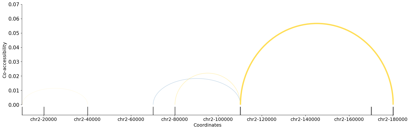
5. Plot co-accessibility scores in a window

You can pass either your anndata object or your freshly extracted dataframe into plot_connections to visualize all Circe scores.
Blue edges correspond to positive co-accessibility scores, while yellow ones are for negative scores

ci.plot_connections(
    circe_network,
    chromosome="chr2",
    start=10_000,
    end=200_000,
    sep=("_","_"),
    abs_threshold=0.01
)

ci.plot_connections(
    atac,
    chromosome="chr2",
    start=10_000,
    end=200_000,
    sep=("_","_"),
    abs_threshold=0.01
)

6. Find cis-coaccessible connected modules

In addition to pairwise co-accessibility scores, Circe can also be used to define cis co-accessibility modules (called CCANs by Cicero), which are modules of sites that are highly co-accessible with one another. We use the Louvain community detection algorithm (Blondel et al., 2008) to find clusters of sites that tended to be co-accessible.

• The function find_ccans takes as input a connection data frame or the anndata object once again, and outputs a data frame with CCAN assignments for each input peak.
  

• You can also use add_ccans to directly add CCAN assignments to your anndata object as anndata.var['CCAN']. The regions that aren’t assigned to a CCAN will contain None.

ccans = ci.find_ccans(circe_network, seed=0)
ccans.head(3)

Coaccessibility cutoff used: 0.0
Number of CCANs generated: 160

	Peak	CCAN
0	chr3_3180001_3180400	1
1	chr3_3220001_3220400	1
2	chr3_3170001_3170400	1

atac = ci.add_ccans(atac, seed=0)

Coaccessibility cutoff used: 0.0

atac.var['CCAN'].value_counts().head(3)

CCAN
24     15
164    15
45     15
Name: count, dtype: int64

With default coaccess_cutoff_override=None, the function will determine and report an appropriate co-accessibility score cutoff value for CCAN generation based on the number of overall CCANs at varying cutoffs. You can also set coaccess_cutoff_override to be a numeric between 0 and 1, to override the cutoff-finding part of the function. This option is useful if you feel that the cutoff found automatically was too strict or loose, or for speed if you are rerunning the code and know what the cutoff will be, since the cutoff finding procedure can be slow.

ccans = ci.find_ccans(circe_network, seed=0, coaccess_cutoff_override=1e-7)

Coaccessibility cutoff used: 1e-07
Number of CCANs generated: 41

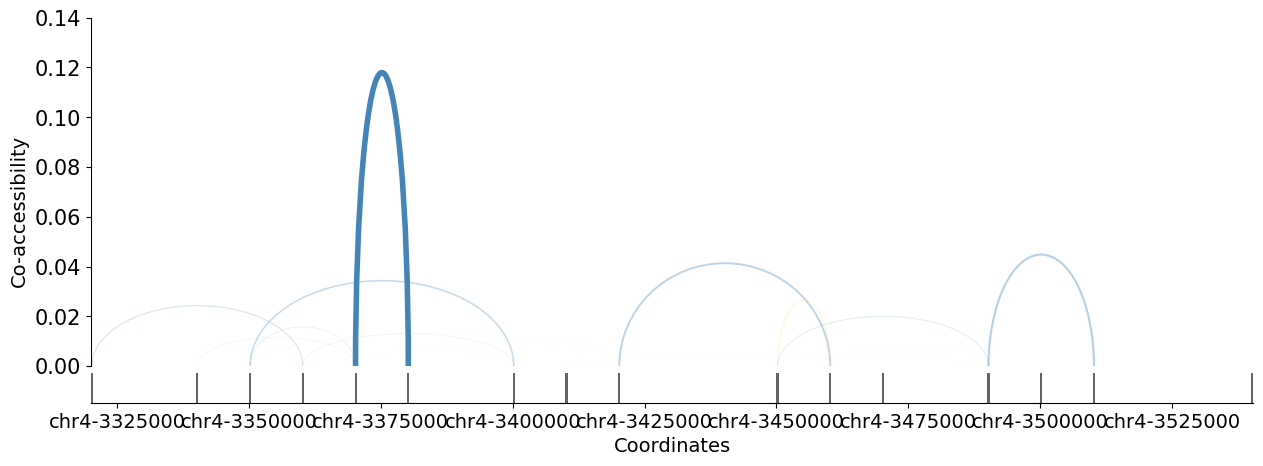
6.B. Plot only a CCAN module

If you’re interested in a specific CCAN module, you can use circe.draw.plot_ccan function, precising its CCAN name. Only the connections between regions belonging to this CCAN module will be plotted.

ci.draw.plot_ccan(
    atac,
    ccan_module=atac.var['CCAN'].value_counts().index[1],
    sep=('_', '_'),
    abs_threshold=0,
    figsize=(15,5),
    only_positive=False)

This CCAN module is on the chromosome: chr4

/home/rtrimbou/ATACNet/circe/circe/draw.py:244: UserWarning: varp parameter is ignored for DataFrame input.
  warnings.warn(

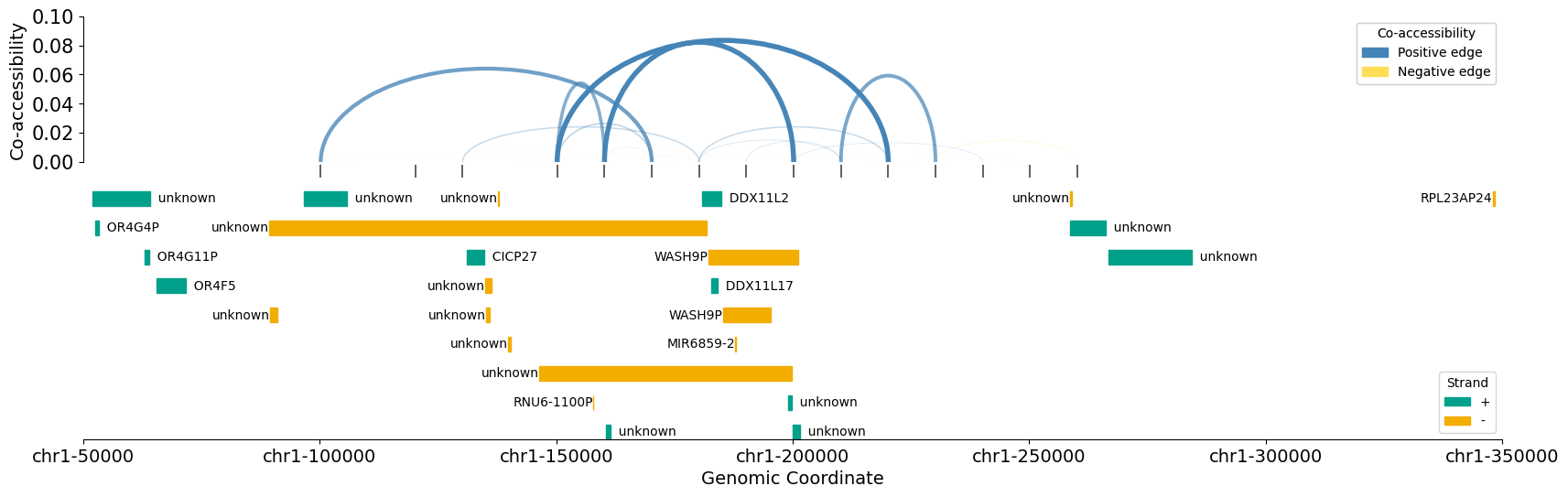
7.Coordinates overlap between co-accessible regions and gene bodies

To better understand the role of specific regions and modules, you can additionally plot gene bodies falling into your window of interest.
You need first to load gene coordinates as a dataframe, or to download them through circe.downloads.download_genes. This functions will require to install the pybiomart package Then you can use ci.draw.plot_connections_genes, using gene infos and either your AnnData object or the dataframe of Circe’s results to compare these locations.

pip install pybiomart

import circe.downloads
genes_df = ci.downloads.download_genes()

import matplotlib.pyplot as plt
fig, ax = plt.subplots(1, figsize = (20, 6))
ci.draw.plot_connections_genes(
    connections=atac,
    genes=genes_df,
    chromosome="chr1",
    start=50_000,
    end=350_000,
    gene_spacing=30_000,
    y_lim_top=-0.01,
    abs_threshold=0.0,
    track_spacing=0.01,
    track_width=0.01,
    legend=True,
    ax=ax
)

7. Work in progress! Happy to get feedbacks :)

If you feel any function could be useful for you on others, don’t hesitate to write me at remi.trimbour@inria.fr or to submit an issue on github.com/cantinilab/Circe.