3. Building CellOracle base-GRN with CIRCE
# pip celloracle
# pip muon
# pip circe
The base GRN of CellOracle are based on cis-accesibility networks obtained from scATAC-seq data. CIRCE now allows users to build the base GRN using a single Python environment.
When CellOracle got published, Cicero, implemented in R, was the current state-of-the-art method to obtain these networks. (Tutorial: base GRN CellOracle¹)
import celloracle as co
which: no R in (/opt/gensoft/exe/Jupyter-Notebook/7.4.4/venv/bin:/opt/gensoft/exe/bedtools/2.31.1/scripts:/opt/gensoft/exe/bedtools/2.31.1/bin:/opt/gensoft/exe/Jupyter-Notebook/7.4.4/bin:/opt/gensoft/adm/Modules/bin:/opt/gensoft/adm/Modules/4.4.0/bin:/opt/hpc/slurm/current/bin:/opt/hpc/slurm/current/sbin:/opt/gensoft/exe/apptainer/1.3.5/scripts:/opt/gensoft/exe/apptainer/1.3.5/bin:/opt/gensoft/exe/apptainer/1.4.1/scripts:/opt/gensoft/exe/apptainer/1.4.1/bin:/opt/gensoft/exe/gcc/10.4.0/bin:/pasteur/appa/homes/rtrimbou/miniconda3/envs/snakemake/bin:/pasteur/appa/homes/rtrimbou/miniconda3/envs/snakemake/condabin:/pasteur/appa/homes/rtrimbou/.local/bin:/pasteur/appa/homes/rtrimbou/bin:/opt/gensoft/adm/Modules/bin:/opt/hpc/slurm/current/bin:/opt/hpc/slurm/current/sbin:/usr/local/bin:/usr/bin:/usr/local/sbin:/usr/sbin)
1. Importing scATAC-seq data
import muon as mu
import circe as ci
The data of this tutorial can be downloaded from this Zenodo repository If you have any trouble to install both CellOracle and CIRCE in the same environement, you try this conda env configuration : CIRCE+CellOracle
data = mu.read_h5mu("pbmc10x/pbmc10x.h5mu")
2. Inferring DNA regions network from CIRCE
atac = data["atac"]
atac, atac.var_names[:3]
atac.var_names = atac.var_names.str.replace('-', '_')
atac = ci.add_region_infos(atac, sep=('_', '_'))
2.a. Computing CIRCE metacells
#atac = ci.metacells.compute_metacells(atac)
2.b. Inferring DNA region interactions
ci.compute_atac_network(atac)
Calculating alpha ━━━━━━━━━━━━━━━━━━━━━━━━━━━━━━━━━━━━━━━━ 0:00:45 0:00:00
2025-09-19 09:12:45,763 - INFO - Remove client Client-e3ecd7f5-9527-11f0-a7a7-3ceceff9f2fe
2025-09-19 09:12:45,767 - INFO - Received 'close-stream' from tcp://127.0.0.1:48784; closing.
2025-09-19 09:12:45,768 - INFO - Remove client Client-e3ecd7f5-9527-11f0-a7a7-3ceceff9f2fe
2025-09-19 09:12:45,769 - INFO - Close client connection: Client-e3ecd7f5-9527-11f0-a7a7-3ceceff9f2fe
2025-09-19 09:12:45,771 - INFO - Retire worker addresses (stimulus_id='retire-workers-1758265965.7718186') (0,)
2025-09-19 09:12:45,781 - INFO - Received 'close-stream' from tcp://127.0.0.1:48782; closing.
2025-09-19 09:12:45,781 - INFO - Remove worker addr: tcp://127.0.0.1:36253 name: 0 (stimulus_id='handle-worker-cleanup-1758265965.7818978')
2025-09-19 09:12:45,782 - INFO - Lost all workers
2025-09-19 09:12:46,305 - INFO - Closing scheduler. Reason: unknown
2025-09-19 09:12:46,306 - INFO - Scheduler closing all comms
Calculating co-accessibility scores...
Concatenating results from all chromosomes...
2.c. Formating network output
circe_network = ci.extract_atac_links(atac)
circe_network = circe_network.rename(
    columns = {"score": "coaccess"}
)
circe_network
| Peak1 | Peak2 | coaccess | |
|---|---|---|---|
| 0 | chr16_54012525_54013025 | chr16_54013534_54014034 | 0.669024 |
| 1 | chr3_133264089_133264589 | chr3_133264946_133265446 | 0.602914 |
| 2 | chr2_109479794_109480294 | chr2_109481034_109481534 | 0.467789 |
| 3 | chr5_49599487_49599987 | chr5_49600285_49600785 | 0.452878 |
| 4 | chr2_88192716_88193216 | chr2_88193738_88194238 | 0.446659 |
| ... | ... | ... | ... |
| 6129848 | chr9_129777081_129777581 | chr9_129869007_129869507 | -0.146761 |
| 6129849 | chr22_38570096_38570596 | chr22_38953902_38954402 | -0.148798 |
| 6129850 | chr18_48896769_48897269 | chr18_48940694_48941194 | -0.148916 |
| 6129851 | chr22_50469821_50470321 | chr22_50542441_50542941 | -0.150171 |
| 6129852 | chr17_82126673_82127173 | chr17_82216598_82217098 | -0.162922 |
6129853 rows × 3 columns
3. Connecting DNA region to gene bodies
This notebook section correspond to the CellOracle documentation: Annotate Transcription Starting Sites²
3.1. TSS informations
!module load bedtools
⚠️You need to have bedtools available !
Otherwise, you should encounter
NotImplementedError: "intersectBed" does not appear to be installed or on the path, so this method is disabled. Please install a more recent version of BEDTools and re-import to use this method.
If you’re on a HPC, you might just have to load the package before launching the notebook: module load bedtools
from celloracle import motif_analysis as ma
# Make sure to specify the correct reference genome here
tss_annotated = ma.get_tss_info(peak_str_list=atac.var_names.values, ref_genome="hg19")

# Check results
tss_annotated.tail()
que bed peaks: 215676
tss peaks in que: 6780
| chr | start | end | gene_short_name | strand | |
|---|---|---|---|---|---|
| 6775 | chr17 | 4834120 | 4834620 | GP1BA | + |
| 6776 | chr17 | 4835384 | 4835884 | GP1BA | + |
| 6777 | chr19 | 35484635 | 35485135 | GRAMD1A | + |
| 6778 | chr7 | 100545748 | 100546248 | MUC3A | + |
| 6779 | chr7 | 100546509 | 100547009 | MUC3A | + |
3.2. Integrating TSS informations with cis-coaccessible network
integrated = ma.integrate_tss_peak_with_cicero(
    tss_peak=tss_annotated,
    cicero_connections=circe_network)
print(integrated.shape)
integrated.head()
(173536, 3)
| peak_id | gene_short_name | coaccess | |
|---|---|---|---|
| 0 | chr10_101291541_101292041 | LINC01475 | 1.000000 |
| 1 | chr10_101291541_101292041 | NKX2-3 | 1.000000 |
| 2 | chr10_101292051_101292551 | LINC01475 | 0.145072 |
| 3 | chr10_101292051_101292551 | NKX2-3 | 1.000000 |
| 4 | chr10_101297817_101298317 | LINC01475 | 0.000032 |
3.3. Filtering peak connections on a specific threshold
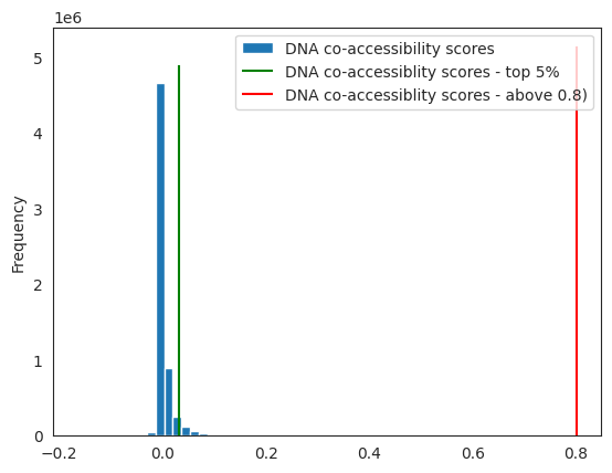
⚠️ As noted in Nourisa et al, 2024 - bioXriv, the threshold of 0.8 might be too high to keep any enhancer - promoter connections.
You can plot the distribution of your score, to realise how many connections you’re keeping.
import matplotlib.pyplot as plt
%matplotlib inline
default_threshold = 0.8

threshold = circe_network.coaccess.quantile(0.95) # TO CHOOSE, e.g. 5% of the connections

fig, ax = plt.subplots(1)
circe_network.coaccess.plot.hist(ax=ax, bins=50, label="DNA co-accessibility scores")  # score distribution
ax.vlines(threshold, 0, ax.get_ylim()[1], colors="green", label="DNA co-accessiblity scores - top 5%")  # threshold line
ax.vlines(default_threshold, 0, ax.get_ylim()[1], colors="red", label="DNA co-accessiblity scores - above 0.8)")  # threshold line
plt.legend()
<matplotlib.legend.Legend at 0x7f40c5d5ca30>
peaks = integrated[integrated.coaccess >= threshold]
peaks = peaks[["peak_id", "gene_short_name"]].reset_index(drop=True)
4. Finding TF binding sites
import celloracle as co
from celloracle import motif_analysis as ma
from celloracle.utility import save_as_pickled_object
co.__version__
'0.20.0'
4.1. Downloading genome - UCSC version
You need a genome sequence in order to identify the TF motifs present in the DNA regions. Genomepy manage the installation by default, but you can also
import genomepy

# This link should be your genome of interest location.
fa = "https://hgdownload.soe.ucsc.edu/goldenPath/hg19/bigZips/latest/hg19.fa.gz"

genomepy.install_genome(
    name=fa,
    provider="URL",
    localname="hg19",
)
Fasta("/pasteur/appa/homes/rtrimbou/.local/share/genomes/hg19/hg19.fa")
⚠️ If your reference genome file are installed in non-default location, please speficy the location using the parameter genomes_dir in the following functions.
Check that the genome has been well downloaded.
# Make sure reference genome has been correctly installed.
ref_genome = "hg19"

genome_installation = ma.is_genome_installed(ref_genome=ref_genome,
                                             genomes_dir=None)
print(ref_genome, "installation: ", genome_installation)
hg19 installation: True
peaks = ma.check_peak_format(peaks, ref_genome, genomes_dir=None)
Peaks before filtering:  20089
Peaks with invalid chr_name:  0
Peaks with invalid length:  0
Peaks after filtering:  20089
4.2. Scanning for TF motifs
# Instantiate TFinfo object
tfi = ma.TFinfo(peak_data_frame=peaks,
                ref_genome=ref_genome,
                genomes_dir=None)
%%time
# Scan motifs. !!CAUTION!! This step may take several hours if you have many peaks!
tfi.scan(fpr=0.02,
         motifs=None,  # If you enter None, default motifs will be loaded.
         verbose=True)

# Save tfinfo object
tfi.to_hdf5(file_path="test1.celloracle.tfinfo")
No motif data entered. Loading default motifs for your species ...
 Default motif for vertebrate: gimme.vertebrate.v5.0.
 For more information, please see https://gimmemotifs.readthedocs.io/en/master/overview.html

Initiating scanner...
2025-09-19 09:28:31,050 - DEBUG - using background: genome hg19 with size 200
Calculating FPR-based threshold. This step may take substantial time when you load a new ref-genome. It will be done quicker on the second time.

Motif scan started .. It may take long time.
CPU times: user 7min 1s, sys: 5.29 s, total: 7min 7s
Wall time: 7min 14s
# Check motif scan results
tfi.scanned_df.head()
| seqname | motif_id | factors_direct | factors_indirect | score | pos | strand | |
|---|---|---|---|---|---|---|---|
| 0 | chr10_101291541_101292041 | GM.5.0.RFX.0001 | Rfx5 | ARID2, Rfx6, Rfx8, RFX6, Rfx3, RFX5, RFX8, Rfx... | 10.484102 | 260 | 1 |
| 1 | chr10_101291541_101292041 | GM.5.0.Nuclear_receptor.0005 | NR4A2, NR1A4, RXRA, NR1H4, FXR | Nr1h5, Nr1h4, Nr1h3, NR1H3 | 8.070402 | 454 | -1 |
| 2 | chr10_101291541_101292041 | GM.5.0.Nuclear_receptor.0005 | NR4A2, NR1A4, RXRA, NR1H4, FXR | Nr1h5, Nr1h4, Nr1h3, NR1H3 | 7.774184 | 454 | 1 |
| 3 | chr10_101291541_101292041 | GM.5.0.Mixed.0008 | ZBTB33, NR2C2 | 9.322807 | 448 | 1 | |
| 4 | chr10_101291541_101292041 | GM.5.0.C2H2_ZF.0020 | Egr1, EGR4, EGR2, Egr3, EGR3, EGR1 | Egr1, Egr4, EGR4, EGR2, Egr3, EGR3, EGR1 | 5.976515 | 124 | 1 |
3.3. Filtering low score TF - peak links
# Reset filtering
tfi.reset_filtering()

# Do filtering
tfi.filter_motifs_by_score(threshold=10)

# Format post-filtering results.
tfi.make_TFinfo_dataframe_and_dictionary(verbose=True)
Filtering finished: 2673574 -> 581057
1. Converting scanned results into one-hot encoded dataframe.
2. Converting results into dictionaries.
4.4. Transforming results into a TF x (peak, gene) dataframe
df = tfi.to_dataframe()
df.head()
| peak_id | gene_short_name | 9430076C15RIK | AC002126.6 | AC012531.1 | AC226150.2 | AFP | AHR | AHRR | AIRE | ... | ZNF784 | ZNF8 | ZNF816 | ZNF85 | ZSCAN10 | ZSCAN16 | ZSCAN22 | ZSCAN26 | ZSCAN31 | ZSCAN4 | |
|---|---|---|---|---|---|---|---|---|---|---|---|---|---|---|---|---|---|---|---|---|---|
| 0 | chr10_101291541_101292041 | LINC01475 | 0.0 | 0.0 | 0.0 | 0.0 | 0.0 | 0.0 | 0.0 | 0.0 | ... | 0.0 | 0.0 | 0.0 | 0.0 | 0.0 | 0.0 | 0.0 | 0.0 | 0.0 | 0.0 |
| 1 | chr10_101291541_101292041 | NKX2-3 | 0.0 | 0.0 | 0.0 | 0.0 | 0.0 | 0.0 | 0.0 | 0.0 | ... | 0.0 | 0.0 | 0.0 | 0.0 | 0.0 | 0.0 | 0.0 | 0.0 | 0.0 | 0.0 |
| 2 | chr10_101292051_101292551 | LINC01475 | 0.0 | 0.0 | 0.0 | 0.0 | 0.0 | 0.0 | 0.0 | 0.0 | ... | 0.0 | 0.0 | 0.0 | 0.0 | 0.0 | 0.0 | 0.0 | 0.0 | 0.0 | 0.0 |
| 3 | chr10_101292051_101292551 | NKX2-3 | 0.0 | 0.0 | 0.0 | 0.0 | 0.0 | 0.0 | 0.0 | 0.0 | ... | 0.0 | 0.0 | 0.0 | 0.0 | 0.0 | 0.0 | 0.0 | 0.0 | 0.0 | 0.0 |
| 4 | chr10_101380430_101380930 | SLC25A28 | 0.0 | 0.0 | 0.0 | 0.0 | 0.0 | 0.0 | 0.0 | 0.0 | ... | 0.0 | 0.0 | 0.0 | 0.0 | 0.0 | 0.0 | 0.0 | 0.0 | 0.0 | 0.0 |
5 rows × 1095 columns
5. Saving the CellOracle base GRN
df.to_parquet("base_GRN_dataframe.parquet")
6. Fitting CellOracle GRN
This notebook section follows the CellOracle documentation: GRN model construction and network analysis³
⚠️ We shortened this part of the workflow to demonstrate the use of CIRCE for CellOracle GRN.
For all details on scRNA-seq data preprocessing, please refer to CellOracle - scRNA-seq data preparation.
During both data preprocessing and GRN inference, we make use of an Oracle object. This object leverages its built-in functions to calculate and store all required information for these steps. To start, we create a new Oracle instance and provide it with our gene expression dataset anndata along with the transcription factor information (the base GRN).
rna = data["rna"]
# Random downsampling into 30K cells if the anndata object include more than 30 K cells.
n_cells_downsample = 30000
if rna.shape[0] > n_cells_downsample:
    # Let's dowmsample into 30K cells
    sc.pp.subsample(rna, n_obs=n_cells_downsample, random_state=123)
6.1. Creating the CellOracle object
# Instantiate Oracle object
oracle = co.Oracle()
6.2. Preprocessing RNA data
import scanpy as sc
import numpy as np
from scipy import sparse
# 1) Keep a copy of the *raw counts* in a layer
rna.layers["raw_count"] = rna.X.copy()
# 2) (Optional) Now you can normalize/log for your own analyses without touching raw_count
sc.pp.normalize_total(rna, target_sum=1e4)
sc.pp.log1p(rna)
# 2.a) Keep the normalized counts in a layer
rna.layers["normalized_count"] = rna.X.copy()
# 3) Neighbors + clustering for 'louvain_annot'
sc.pp.pca(rna)
sc.pp.neighbors(rna)
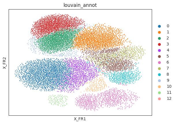
sc.tl.louvain(rna, key_added="louvain_annot") # or sc.tl.leiden(..., key_added="louvain_annot")
rna.obs["louvain_annot"] = rna.obs["louvain_annot"].astype("category")
# 4) ForceAtlas2 embedding (Scanpy's draw_graph)
sc.tl.draw_graph(rna) # creates rna.obsm["X_draw_graph_fa"]
# 5) Point .X to the unscaled counts for Oracle (optional, Oracle will read from layers below)
rna.X = rna.layers["raw_count"].copy()
# 6) Import to Oracle
oracle.import_anndata_as_raw_count(
adata=rna,
cluster_column_name="louvain_annot",
embedding_name="X_draw_graph_fr",
)
WARNING: adata.X seems to be already log-transformed.
WARNING: Package 'fa2-modified' is not installed, falling back to layout 'fr'.To use the faster and better ForceAtlas2 layout, install package 'fa2-modified' (`pip install fa2-modified`).
18410 genes were found in the adata. Note that Celloracle is intended to use around 1000-3000 genes, so the behavior with this number of genes may differ from what is expected.
WARNING: adata.X seems to be already log-transformed.
6.3. Loading prior base GRN
# You can load TF info dataframe with the following code.
oracle.import_TF_data(TF_info_matrix=df)
TF dict already exists. The old TF dict data was deleted.
6.4. Calculating KNN for cell proximity and trajectories
Compute PCA and select a small number of components.
# Perform PCA
oracle.perform_PCA()

# Select important PCs
plt.plot(np.cumsum(oracle.pca.explained_variance_ratio_)[:100])
n_comps = np.where(np.diff(np.diff(np.cumsum(oracle.pca.explained_variance_ratio_))>0.002))[0][0]
plt.axvline(n_comps, c="k")
plt.show()
print(n_comps)
n_comps = min(n_comps, 50)
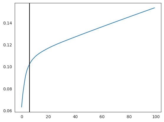
6
Defining a number of neighbors for KNN imputation.
n_cell = oracle.adata.shape[0]
print(f"cell number is :{n_cell}")

k = int(0.025*n_cell)
print(f"Auto-selected k is :{k}")
cell number is :9631
Auto-selected k is :240
Computing k-nearest neighbors.
oracle.knn_imputation(n_pca_dims=n_comps, k=k, balanced=True, b_sight=k*8,
                      b_maxl=k*4, n_jobs=4)
# Check clustering data
sc.pl.draw_graph(oracle.adata, color="louvain_annot")
6.5. Inferring cluster-specific GRN
%%time
# Calculate GRN for each population in "louvain_annot" clustering unit.
# This step may take some time.(~30 minutes)
links = oracle.get_links(cluster_name_for_GRN_unit="louvain_annot", alpha=10,
                         verbose_level=10)
Inferring GRN for 0...
Inferring GRN for 1...
Inferring GRN for 10...
Inferring GRN for 11...
Inferring GRN for 12...
Inferring GRN for 2...
Inferring GRN for 3...
Inferring GRN for 4...
Inferring GRN for 5...
Inferring GRN for 6...
Inferring GRN for 7...
Inferring GRN for 8...
Inferring GRN for 9...
CPU times: user 1h 22min 15s, sys: 4min 40s, total: 1h 26min 55s
Wall time: 1h 48min 31s
!conda env export > circe_celloracle_env.yml